User Guide#

This user guide will showcase the capabilities of PedPy. By following this guide you will learn how to set up your analysis and compute different metrics from the movement data. This guide is designed as a Jupyter notebook where the individual cells can be executed in the given order, for trying it yourself you can copy the individual cells in a Python script and run it, or download the notebook here it directly and run it locally.

If you use PedPy in your work, please cite it using the following information from zenodo:

This is a bottleneck experiment conducted at the University of Wuppertal in 2018. You can see the basic setup of the experiment in the picture below:

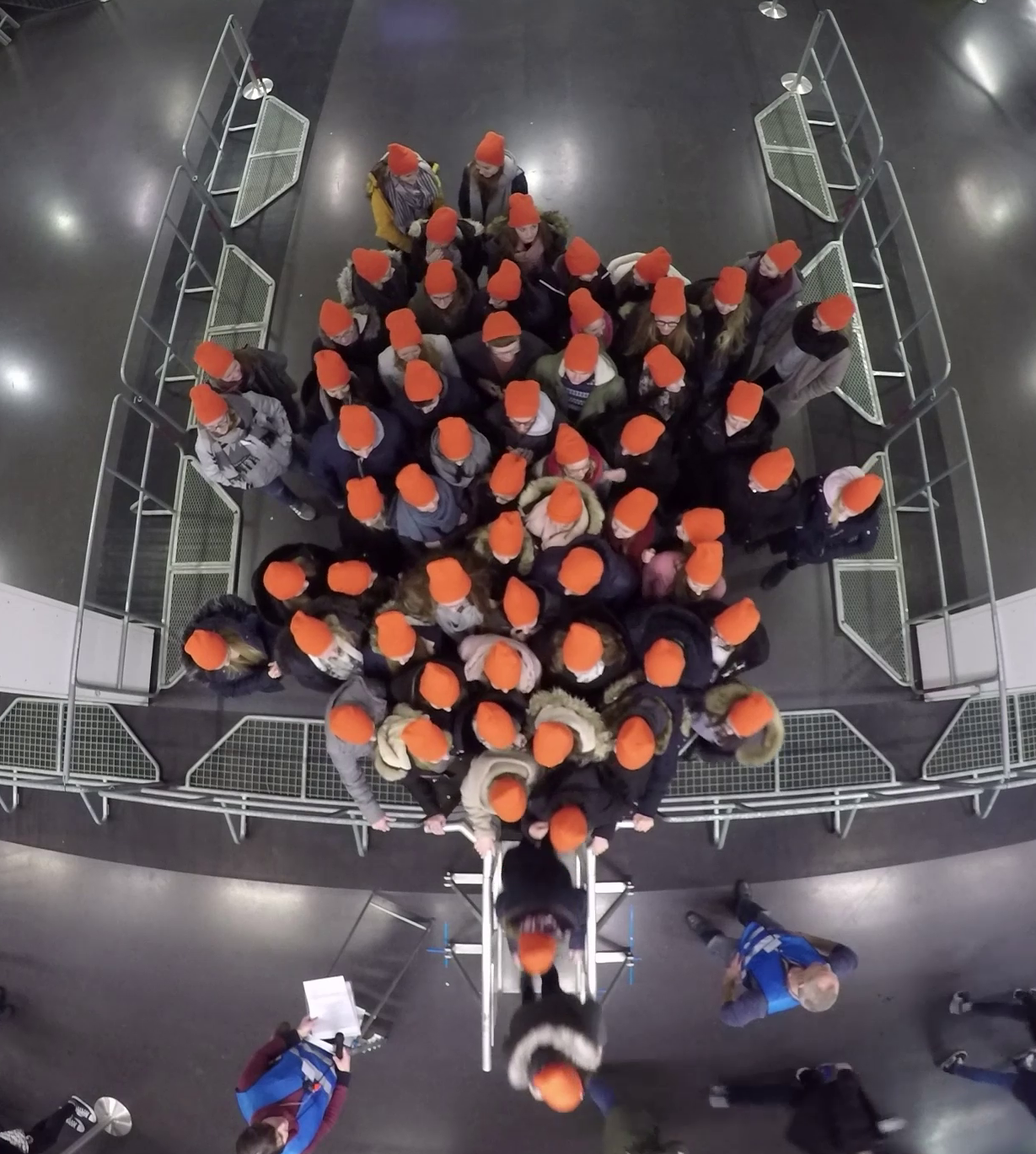
The data for this experiment is available here, which belongs to this experimental series and is part of the publication “Crowds in front of bottlenecks at entrances from the perspective of physics and social psychology”.

Analysis set-up#

The first step we will take, is to set up the analysis environment, this means define the areas where pedestrians can walk and put existing obstacles in it. Also, we will define which areas are of interest for the later analysis.

Walkable area#

In the beginning we will define the walkable area in which the pedestrian can move. For the used bottleneck experiment was conducted in the following set up:

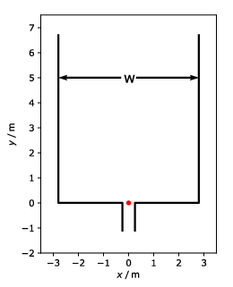
The run handled in this user guide had a bottleneck width of 0.5m and w=5.6m.

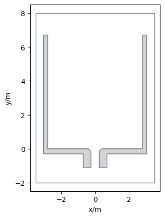
Below is the code for creating such a walkable area:

from pedpy import WalkableArea

walkable_area = WalkableArea(
    # complete area
    [
        (3.5, -2),
        (3.5, 8),
        (-3.5, 8),
        (-3.5, -2),
    ],
    obstacles=[
        # left barrier
        [
            (-0.7, -1.1),
            (-0.25, -1.1),
            (-0.25, -0.15),
            (-0.4, 0.0),
            (-2.8, 0.0),
            (-2.8, 6.7),
            (-3.05, 6.7),
            (-3.05, -0.3),
            (-0.7, -0.3),
            (-0.7, -1.0),
        ],
        # right barrier
        [
            (0.25, -1.1),
            (0.7, -1.1),
            (0.7, -0.3),
            (3.05, -0.3),
            (3.05, 6.7),
            (2.8, 6.7),
            (2.8, 0.0),
            (0.4, 0.0),
            (0.25, -0.15),
            (0.25, -1.1),
        ],
    ],
)

_images/a30ae7a4d7f150ac6c8eec62e16225b42da092d269db4d9e3ecf658ed05315c8.png

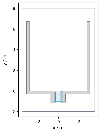
Prepare measurement details#

After we defined where the pedestrians can move, we now need to define in which regions we want to analyze in more details. This regions can either be a specific line, an area, or the whole walkable area.

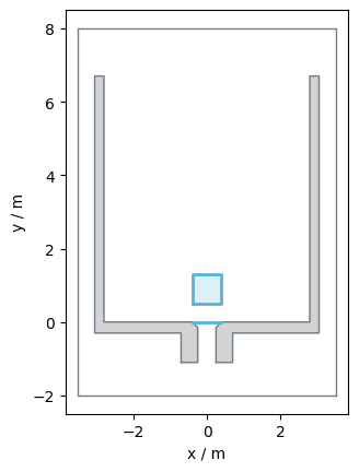
In case of this bottleneck the most interesting area is a little bit in front of the bottleneck (here 0.5m) and the line at the beginning of the bottleneck. The area is slightly in front of the bottleneck as here the highest density occur. In PedPy such areas are called MeasurementArea and the lines MeasurementLine. Below you can see how to define these:

from pedpy import MeasurementArea, MeasurementLine

measurement_area = MeasurementArea(
    [(-0.4, 0.5), (0.4, 0.5), (0.4, 1.3), (-0.4, 1.3)]
)

measurement_line = MeasurementLine([(0.4, 0), (-0.4, 0)])

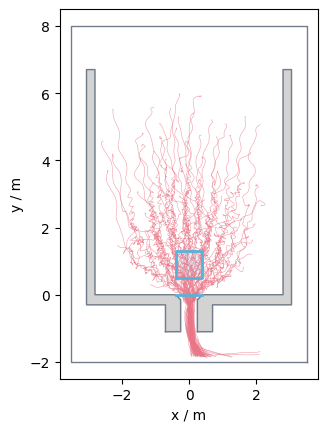
The corresponding measurement setup looks like:

_images/73f44a09620e95913b7a80ce38aee2efc1a9013ea0e5fe8744b7198570cfb08b.png

Importing pedestrian movement data#

The pedestrian movement data in PedPy is called trajectory data.

PedPy works with trajectory data which can be created from an import function for specific data files alternatively from a DataFrame with the following columns:

“id”: unique numeric identifier for each person
“frame”: index of video frame where the positions were extracted
“x”, “y”: position of the person (in meter)

Loading from Pandas DataFrame#

To construct the trajectory data from a DataFrame you also need to provide the frame rate at which the data was recorded. If you have both the construction of the trajectory data can be done with:

from pedpy import TrajectoryData

data = pd.DataFrame(
    [[0, 1, 0, 0]],
    columns=["id", "frame", "x", "y"],
)
trajectory_data = TrajectoryData(data=data, frame_rate=25.0)

Alternatively, the data can be also loaded from any file format that is supported by Pandas, see the documentation for more details.

Loading from text trajectory files#

Pedpy can load trajectories, if they are stored as the trajectory data provided in the Jülich Data Archive directly. If you have text files in same format, you can load them in the same way too:

values are separated by any whitespace, e.g., space, tab
file has at least 4 columns in the following order: “id”, “frame”, “x”, “y”
file may contain comment lines with # at in the beginning

For meaningful analysis (and loading of the trajectory file) you also need

unit of the trajectory (m or cm)
frame rate

For recent trajectory they are encoded in the header of the file, for older you may need to lead the documentation and provide the information in the loading process.

Examples: With frame rate, but no unit

# description: UNI_CORR_500_01
# framerate: 25.00
#geometry: geometry.xml

# PersID	Frame	X	Y	Z
1	98	4.6012	1.8909	1.7600
1	99	4.5359	1.8976	1.7600
1	100	4.4470	1.9304	1.7600
...

No header at all:

27 164.834 780.844 168.937
28 164.835 771.893 168.937
29 163.736 762.665 168.937
30 161.967 753.088 168.937
...

If your data is structured in a different way please take a look at the next section. Since the data we want to analyze is from the data archive, we can directly load the trajectory data with PedPy:

from pedpy import load_trajectory, TrajectoryUnit

traj = load_trajectory(
    trajectory_file=pathlib.Path("demo-data/bottleneck/040_c_56_h-.txt"),
    default_unit=TrajectoryUnit.METER,  # needs to be provided as it not defined in the file
    # default_frame_rate=25., # can be ignored here as the frame rate is defined in the file
)

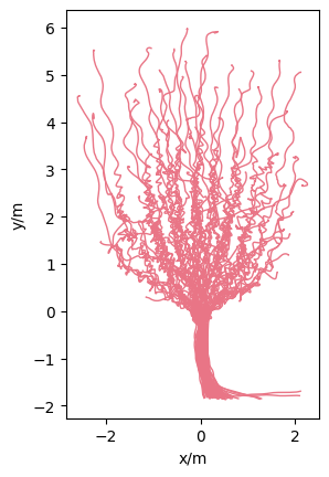
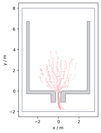
The loaded trajectory data look like:

_images/d8ecc7dbb101f1dda68ce78e51dcd5de61cba0ced797cce34b7ffb894af6c4b3.png

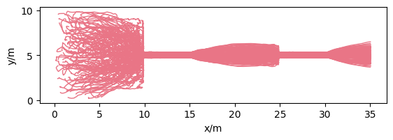
Loading from hdf5 trajectory files#

For some experiments the Jülich Data Archive also provides HDF5 trajectory files, with a structure described here. These data are from a different experiment, and are only used to demonstrate how to load HDF5 files, it can be downloaded here.

To make the data usable for PedPy use:

from pedpy import (
    TrajectoryData,
    load_trajectory_from_ped_data_archive_hdf5,
    load_walkable_area_from_ped_data_archive_hdf5,
)
import pathlib

h5_file = pathlib.Path("demo-data/single_file/00_01a.h5")

traj_h5 = load_trajectory_from_ped_data_archive_hdf5(trajectory_file=h5_file)
walkable_area_h5 = load_walkable_area_from_ped_data_archive_hdf5(
    trajectory_file=h5_file
)

_images/7e118c48e88f10aba832bdb0feaf29ed3c5e44e3f924a5906bf5f381e10f88c2.png

Loading from Viswalk trajectory files#

It is also possible to load trajectory files from Viswalk directly into PedPy. The expected format is a CSV file with ; as delimiter, and it should contain at least the following columns: NO, SIMSEC, COORDCENTX, COORDCENTY. Comment lines may start with a * and will be ignored.

Important

Currently only Viswalk trajectory files, which use the simulation time (SIMSEC) are supported.

To make the data usable for PedPy use:

from pedpy import (
    TrajectoryData,
    load_trajectory_from_viswalk,
)
import pathlib

viswalk_file = pathlib.Path("demo-data/viswalk/example.pp")

traj_viswalk = load_trajectory_from_viswalk(trajectory_file=viswalk_file)

_images/a00fdb94e26b879e01de596f8f149005c605c642cb93dffc69c825522245c3e7.png

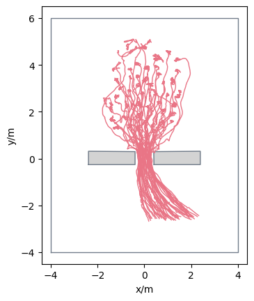
Plot setup#

For a better overview of our created measurement setup, see the plot below:

_images/e81a722ae9c789aea7a3952d7d0b6c957d861b9d5217a19c20940ec660fbf24d.png

Validate that trajectory is completely inside the walkable area.#

An important step before starting the analysis is to verify that all trajectories lie within the constructed walkable area. Otherwise, you might get errors. PedPy provides a function to test your trajectories, and offers also a function to get all invalid trajectories:

from pedpy import is_trajectory_valid, get_invalid_trajectory

print(
    f"Trajectory is valid: {is_trajectory_valid(traj_data=traj, walkable_area=walkable_area)}"
)
get_invalid_trajectory(traj_data=traj, walkable_area=walkable_area)

Trajectory is valid: True

	id	frame	x	y	point

For demonstration purposes, wrongly place the obstacle s.th. some pedestrian walk through it!

We now create a faulty geometry, s.th. you can see how the result would like. Therefore, the right obstacle will be moved a bit towards the center of the bottlneck:

_images/b9827490dc3f86e3e269f8a2b888fc9956049174173a58f9740039c6d4befdb8.png

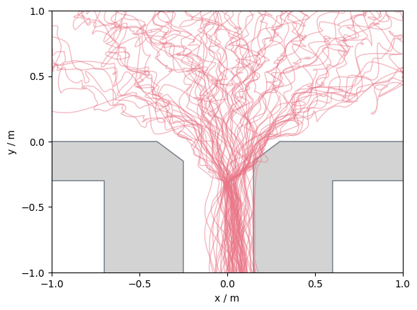
If you get any invalid trajectories, you should check whether you constructed your walkable area correctly. In some cases you will get such errors when you have head trajectories, and the pedestrian lean over the obstacles. Then you need to prepare your data before you can start your analysis.

from pedpy import is_trajectory_valid, get_invalid_trajectory

print(
    f"Trajectory is valid: {is_trajectory_valid(traj_data=traj, walkable_area=walkable_area_faulty)}"
)
get_invalid_trajectory(traj_data=traj, walkable_area=walkable_area_faulty)

Trajectory is valid: False

	id	frame	x	y	point
2653	4	642	0.1683	-0.1333	POINT (0.1683 -0.1333)
2654	4	643	0.1708	-0.1462	POINT (0.1708 -0.1462)
2655	4	644	0.1727	-0.1592	POINT (0.1727 -0.1592)
2656	4	645	0.1658	-0.1622	POINT (0.1658 -0.1622)
2657	4	646	0.1586	-0.1626	POINT (0.1586 -0.1626)
...	...	...	...	...	...
36685	49	1253	0.1545	-0.9367	POINT (0.1545 -0.9367)
36686	49	1254	0.1554	-0.9680	POINT (0.1554 -0.968)
36687	49	1255	0.1581	-1.0000	POINT (0.1581 -1)
36688	49	1256	0.1622	-1.0331	POINT (0.1622 -1.0331)
36689	49	1257	0.1693	-1.0671	POINT (0.1693 -1.0671)

103 rows × 5 columns

Analysis#

Now that we set up the analysis environment, we can start with the real analysis. PedPy provides different methods to obtain multiple metric from the trajectory data:

Density
Speed
Flow
Neighborhood
Distance/Time to entrance
Profiles

Density#

Density is a fundamental metric in pedestrian dynamics. As it indicated how much space is accessible to each pedestrian within a specific area. High density can lead to reduced walking speeds, increased congestion, and even potential safety hazards.

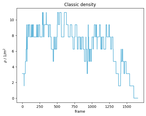
Classic density#

The classic approach to calculate the density \(\rho_{classic}(t)\) at a time \(t\), is to count the number of pedestrians (\(N(t)\)) inside a specific space (\(M\)) and divide it by the area of that space (\(A(M)\)).

\[ \rho_{classic}(t) = {N(t) \over A(M)} \]

In PedPy this can be computed with:

from pedpy import compute_classic_density

classic_density = compute_classic_density(
    traj_data=traj, measurement_area=measurement_area
)

The resulting time-series can be seen below:

_images/dee339ced4b50724f6c740bb600497199eaf7ae27d65e0cba31c035e87e4fc91.png

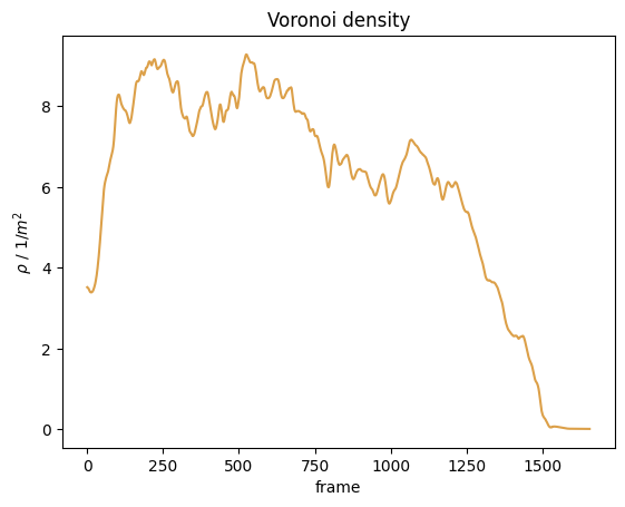
Voronoi density#

Another approach for calculating the density is to compute the Voronoi tesselation of the pedestrians positions at a given time \(t\), the resulting Voronoi polygons (\(V\)) directly relate to the individual’s density. For a pedestrian \(i\) the individual density is defined as:

\[ \rho_i(t) = {1 \over A(V_i(t)} \]

Compute individual Voronoi Polygons#

The first step for computing the Voronoi density, is to compute the individual’s Voronoi polygon. As these polygons may become infinite for pedestrians at the edge of the crowd, these polygons are restricted by the walkable area. This cutting at the boundaries can lead to split Voronoi polygons. For each of the split polygons it is checked, in which the pedestrian is located. This polygon then is assigned.

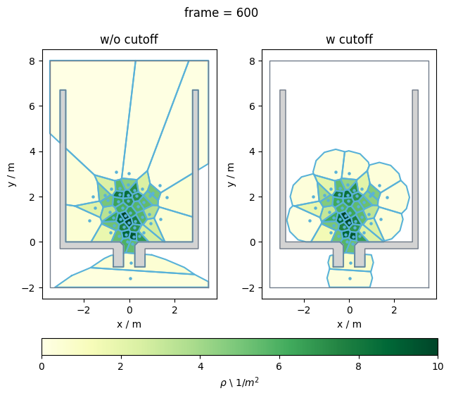
Important

As these Voronoi polygons work on the Euclidean distance, some unexpected artifacts may occur on non-convex walkable areas. Please keep that in mind! How that may look like, you can see in the plots later in this guide.

Without cut-off#

The computation of the individual polygons can be done from the trajectory data and walkable area with:

from pedpy import compute_individual_voronoi_polygons

individual = compute_individual_voronoi_polygons(
    traj_data=traj, walkable_area=walkable_area
)

With cut-off#

When having a large walkable area or widely spread pedestrians the Voronoi polygons may become quite large. In PedPy it is possible to restrict the size of the computed Polygons. This can be done by defining a cut off, which is essentially an approximated circle which gives the maximum extension of a single Voronoi polygon. For the creation of the cut off, we need to define how accurate we want to approximate the circle, the differences can be seen below:

Now, with that cut off the computation of the individual polygons becomes:

from pedpy import compute_individual_voronoi_polygons, Cutoff

individual_cutoff = compute_individual_voronoi_polygons(
    traj_data=traj,
    walkable_area=walkable_area,
    cut_off=Cutoff(radius=1.0, quad_segments=3),
)

Comparison#

To get a better impression what the differences between the Voronoi polygons with and without the cut off are, take a look at the plot below:

_images/bffff844ff96c74d2b6d38a98db14753d42c1ede5a8eb8c2eed9fb59db2c2ad0.png

Compute actual Voronoi density#

From these individual data we can now compute the Voronoi density \(\rho_{voronoi}(t)\) in the known measurement area (\(M\)):

\[ \rho_{voronoi}(t) = { \int\int \rho_{xy}(t) dxdy \over A(M)}, \]

where \(\rho_{xy}(t) = 1 / A(V_i(t))\) is the individual density of each pedestrian, whose \(V_i(t) \cap M\) and \(A(M)\) the area of the measurement area.

Without cut-off#

First, we compute the Voronoi density in the measurement area without a cut off:

from pedpy import compute_voronoi_density

density_voronoi, intersecting = compute_voronoi_density(
    individual_voronoi_data=individual, measurement_area=measurement_area
)

_images/20d92437b57f549ca90cc3254eeaeb9077d4f60bfc7a5ed6a9e4c12adad42074.png

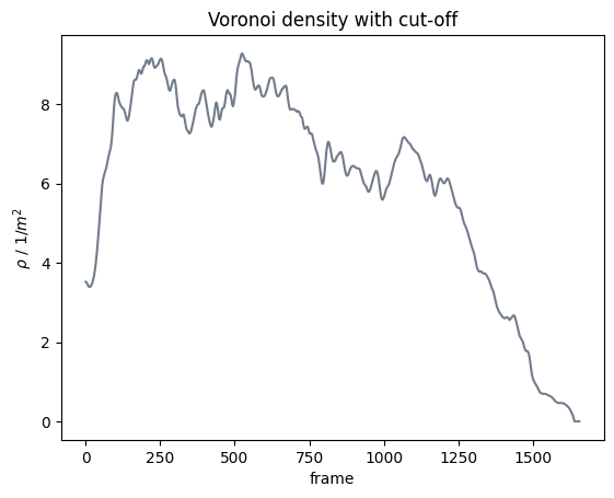
With cut-off#

Second, we compute it now from the individual cut off Voronoi polygons:

from pedpy import compute_voronoi_density

density_voronoi_cutoff, intersecting_cutoff = compute_voronoi_density(
    individual_voronoi_data=individual_cutoff, measurement_area=measurement_area
)

_images/5922759a02e0d0f2a333746133d3990a21e764bb80f194f50937a84b97e8890b.png

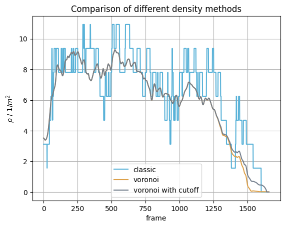
Comparison#

Now we have obtained the mean density inside the measurement area with different methods. To compare the results take a look at the following plot:

_images/e050c01fc2796d4a09c1f554664664c640fdb09cc78c7b1b61eb767ae7275ab5.png

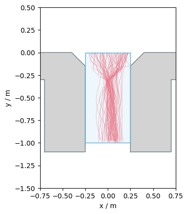
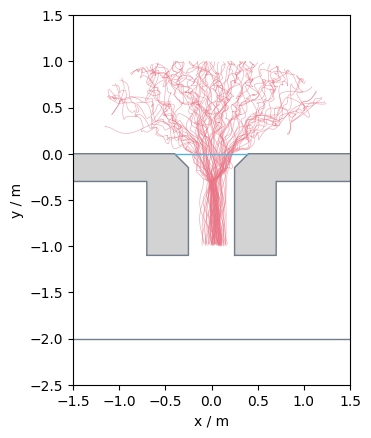
Passing density (individual)#

Another option to compute the individual density, is the passing density. For the computation it needs a measurement line and the distance to a second “virtual” measurement line which form a “virtual” measurement area (\(M\)).

For each pedestrians now the frames when they enter and leave the virtual measurement area is computed. In this frame interval they have to be inside the measurement area continuously. They also need to enter and leave the measurement area via different measurement lines. If leaving the area between the two lines, crossing the same line twice they will be ignored. For a better understanding, see the image below, where red parts of the trajectories are the detected ones inside the area. These frame intervals will be returned.

In this our example, we want to measure from the entrance of the bottleneck (top line) 1m towards the exit of the bottleneck (bottom line). The set-up is shown below:

_images/ac70a470940a32fbb42d2efdc6547d8c21a64f0971f467ce84e4eac5b00e8560.png

The passing density for each pedestrian \(\rho_{passing}(i)\) is the average number of pedestrian who are in the same measurement area \(M\) in the same time interval (\([t_{in}(i), t_{out}(i)]\)) as pedestrian \(i\), divided by the area of that measurement area \(A(M)\).

Then the computation becomes:

\[ \rho_{passing}(i) = {1 \over {t_{out}(i)-t_{in}(i)}} \int^{t_{out}(i)}_{t_{in}(i)} {{N(t)} \over A(M)} dt \]

where \(t_{in}(i) = f_{in}(i) / fps\) is the time the pedestrian crossed the first line and \(t_{out}(i) = f_{out}(i) / fps\) when they crossed the second line, where \(f_{in}\) and \(f_{out}\) are the frames where the pedestrian crossed the first line, and the second line respectively. And \(fps\) is the frame rate of the trajectory data.

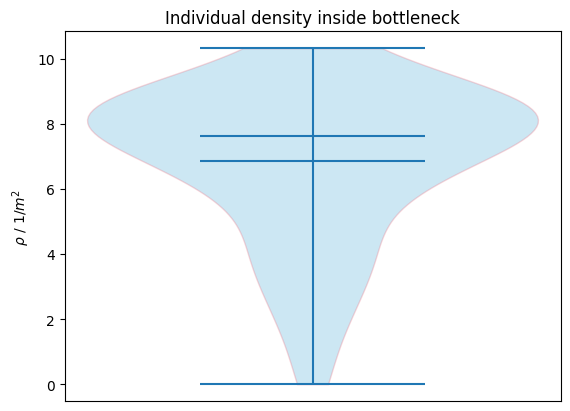
Here, we want to compute the passing density inside the bottleneck, this can be done with:

from pedpy import compute_passing_density
from pedpy import compute_frame_range_in_area

frames_in_area, used_area = compute_frame_range_in_area(
    traj_data=traj, measurement_line=measurement_line, width=1.0
)
passing_density = compute_passing_density(
    density_per_frame=classic_density, frames=frames_in_area
)

This gives for each pedestrian one value for the density. The following plot shows how the individual density inside is distributed the bottleneck:

_images/6fb7a370387574592a220992815b40e4c6e418a0c80d775da2c37f9b4b20b0a6.png

Speed#

A further important measure in pedestrian dynamics is the speed of the pedestrians. Low speeds can indicate congestions or other obstructions in the flow of the crowd.

Individual speed#

For computing the individuals speed at a specific frame \(v_i(t)\), a specific frame step (\(n\)) is needed. Together with the frame rate of the trajectory data \(fps\) the time frame \(\Delta t\) for computing the speed becomes:

\[ \Delta t = 2 n / fps \]

This time step describes how many frames before and after the current position \(X_{current}\) are used to compute the movement. These positions are called \(X_{future}\), \(X_{past}\), respectively.

First computing the displacement between these positions \(\bar{X}\). This then can be used to compute the speed with:

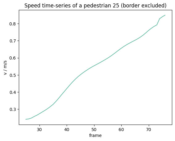
\[\begin{split}\begin{align} \bar{X} &= X_{future} - X_{past} \\ v_i(t) &= \frac{\bar{X}}{\Delta t} \end{align}\end{split}\]

When getting closer to the start, or end of the trajectory data, it is not possible to use the full range of the frame interval for computing the speed. For these cases PedPy offers three different methods to compute the speed:

exclude these parts
adaptively shrink the window in which the speed is computed
switch to one-sided window

Exclude border#

When not enough frames available to compute the speed at the borders, for these parts no speed can be computed and they are ignored.

from pedpy import compute_individual_speed, SpeedCalculation

frame_step = 25

individual_speed_exclude = compute_individual_speed(
    traj_data=traj,
    frame_step=frame_step,
    compute_velocity=True,
    speed_calculation=SpeedCalculation.BORDER_EXCLUDE,
)

_images/5219b49f2ba53a66c76a0ee0759ccc1c41928905fcba7d9a54bd0028f93a89b9.png

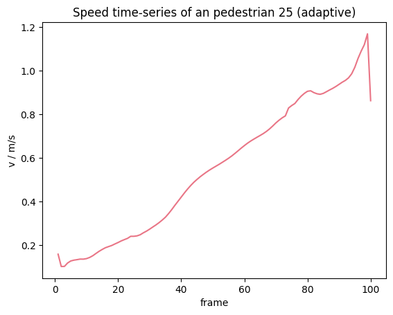
Adaptive border window#

In the adaptive approach, it is checked how many frames \(n\) are available to from \(X_{current}\) to the end of the trajectory. This number is then used on both sides to create a smaller symmetric window, which yields \(X_{past}\) and \(X_{future}\). Now with the same principles as before the individual speed \(v_i(t)\) can be computed.

_images/speed_border_adaptive_future.svg

Important

As the time interval gets smaller to the ends of the individual trajectories, the oscillations in the speed increase here.

from pedpy import compute_individual_speed, SpeedCalculation

individual_speed_adaptive = compute_individual_speed(
    traj_data=traj,
    frame_step=frame_step,
    compute_velocity=True,
    speed_calculation=SpeedCalculation.BORDER_ADAPTIVE,
)

_images/e5142dd875fadb2fd9bbd359862c715cf2004af418e1aff4f9a167b5c9eca288.png

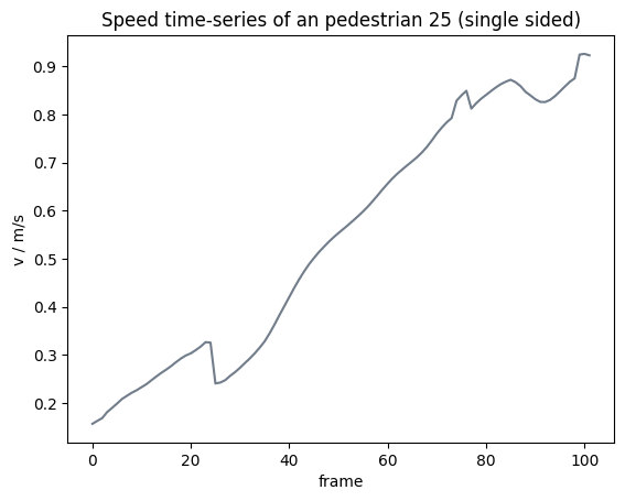
Single sided border window#

In these cases, one of the end points to compute the movement becomes the current position \(X_{current}\). When getting too close to the start of the trajectory, the movement is computed from \(X_{current}\) to \(X_{future}\). In the other case the movement is from \(X_{past}\) to \(X_{current}\).

\[ v_i(t) = {|{X_{future} - X_{current}|}\over{ \frac{1}{2} \Delta t}} \text{, or } v_i(t) = {|{X_{current} - X_{past}|}\over{ \frac{1}{2} \Delta t}} \]

_images/speed_border_single_sided_future.svg

_images/speed_border_single_sided_past.svg

Important

As at the edges of the trajectories the time interval gets halved, there may occur some jumps computed speeds at this point.

from pedpy import compute_individual_speed, SpeedCalculation

individual_speed_single_sided = compute_individual_speed(
    traj_data=traj,
    frame_step=frame_step,
    compute_velocity=True,
    speed_calculation=SpeedCalculation.BORDER_SINGLE_SIDED,
)

_images/81f690e79b2637605ebb65d565029b2a2501fefddb1978c8639dc6a3415d6d35.png

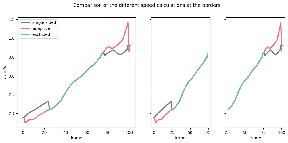
Comparison#

To demonstrate the differences in the computed speeds, take a look at the following plot:

Show code cell source Hide code cell source

from pedpy import PEDPY_GREY, PEDPY_RED, PEDPY_GREEN
import matplotlib.pyplot as plt

fig, ax = plt.subplots(
    1, 3, gridspec_kw={"width_ratios": [2, 1, 1]}, sharey=True, figsize=(12, 5)
)

fig.suptitle("Comparison of the different speed calculations at the borders")
speed_exclude = individual_speed_exclude[individual_speed_exclude.id == ped_id]
speed_adaptive = individual_speed_adaptive[
    individual_speed_adaptive.id == ped_id
]
speed_single_sided = individual_speed_single_sided[
    individual_speed_single_sided.id == ped_id
]

ax[0].plot(
    speed_single_sided.frame,
    speed_single_sided.speed,
    color=PEDPY_GREY,
    linewidth=3,
    label="single sided",
)
ax[0].plot(
    speed_adaptive.frame,
    speed_adaptive.speed,
    color=PEDPY_RED,
    linewidth=3,
    label="adaptive",
)
ax[0].plot(
    speed_exclude.frame,
    speed_exclude.speed,
    color=PEDPY_GREEN,
    linewidth=3,
    label="excluded",
)
ax[0].set_xlabel("frame")
ax[0].set_ylabel("v / m/s")
ax[0].legend()

ax[1].plot(
    speed_single_sided.frame[
        speed_single_sided.frame
        < speed_single_sided.frame.min() + 3 * frame_step
    ],
    speed_single_sided.speed[
        speed_single_sided.frame
        < speed_single_sided.frame.min() + 3 * frame_step
    ],
    color=PEDPY_GREY,
    linewidth=3,
)
ax[1].plot(
    speed_adaptive.frame[
        speed_adaptive.frame < speed_single_sided.frame.min() + 3 * frame_step
    ],
    speed_adaptive.speed[
        speed_adaptive.frame < speed_single_sided.frame.min() + 3 * frame_step
    ],
    color=PEDPY_RED,
    linewidth=3,
)
ax[1].plot(
    speed_exclude.frame[
        speed_exclude.frame < speed_single_sided.frame.min() + 3 * frame_step
    ],
    speed_exclude.speed[
        speed_exclude.frame < speed_single_sided.frame.min() + 3 * frame_step
    ],
    color=PEDPY_GREEN,
    linewidth=3,
)
ax[1].set_xlabel("frame")

ax[2].plot(
    speed_single_sided.frame[
        speed_single_sided.frame
        > speed_single_sided.frame.max() - 3 * frame_step
    ],
    speed_single_sided.speed[
        speed_single_sided.frame
        > speed_single_sided.frame.max() - 3 * frame_step
    ],
    color=PEDPY_GREY,
    linewidth=3,
)
ax[2].plot(
    speed_adaptive.frame[
        speed_adaptive.frame > speed_single_sided.frame.max() - 3 * frame_step
    ],
    speed_adaptive.speed[
        speed_adaptive.frame > speed_single_sided.frame.max() - 3 * frame_step
    ],
    color=PEDPY_RED,
    linewidth=3,
)
ax[2].plot(
    speed_exclude.frame[
        speed_exclude.frame > speed_single_sided.frame.max() - 3 * frame_step
    ],
    speed_exclude.speed[
        speed_exclude.frame > speed_single_sided.frame.max() - 3 * frame_step
    ],
    color=PEDPY_GREEN,
    linewidth=3,
)

ax[2].set_xlabel("frame")
plt.show()

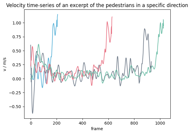
_images/4718410d1d61872509319c6fd7435b348141096a6cf7c52d767fd915325fa24f.png

Individual speed in specific movement direction#

It is also possible to compute the individual speed in a specific direction \(d\), for this the movement \(\bar{X}\) is projected onto the desired movement direction. \(\bar{X}\) and \(\Delta t\) are computed as described above. Hence, the speed then becomes:

\[ v_i(t) = {{|\boldsymbol{proj}_d\; \bar{X}|} \over {\Delta t}} \]

Important

When using a specific direction, the computed speed may become negative.

individual_speed_direction = compute_individual_speed(
    traj_data=traj,
    frame_step=5,
    movement_direction=np.array([0, -1]),
    compute_velocity=True,
    speed_calculation=SpeedCalculation.BORDER_SINGLE_SIDED,
)

_images/745c484033e885f478b4c832f964b0f96fe5c9038856f826ca5fd1361f71808f.png

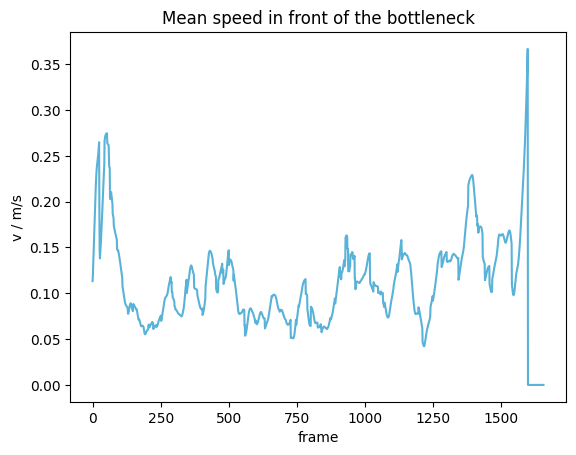
Mean speed#

Now, that we have computed the individual’s speed, we want to compute the mean speed in the already used measurement area \(M\) closely in front of the bottleneck. The mean speed is defined as

\[ v_{mean}(t) = {{1} \over {N}} \sum_{i \in P_M} v_i(t), \]

where \(P_M\) are all pedestrians inside the measurement area, and \(N\) the number of pedestrians inside the measurement area (\(|P_M|\)).

Important

The mean speed can only be computed when for each pedestrian inside the measurement area also a speed \(v_i(t)\) is computed, when using the exclude or adaptive approach this might not be the case. Then some extra processing steps are needed, to avoid this use the single sided approach.

This can be as follows with PedPy:

from pedpy import compute_mean_speed_per_frame

mean_speed = compute_mean_speed_per_frame(
    traj_data=traj,
    measurement_area=measurement_area,
    individual_speed=individual_speed_single_sided,
)

_images/d0af61e521181fff9c381c330fe9c69afd35c17913693204805a273aebb0616f.png

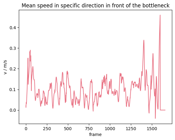
The same can be now computed, using the speed in a movement direction as basis:

mean_speed_direction = compute_mean_speed_per_frame(
    traj_data=traj,
    measurement_area=measurement_area,
    individual_speed=individual_speed_direction,
)

_images/8dedfa2239c14cfbfa67c46de0c668fab55a0c35175a188d1f2c5b9bb306163b.png

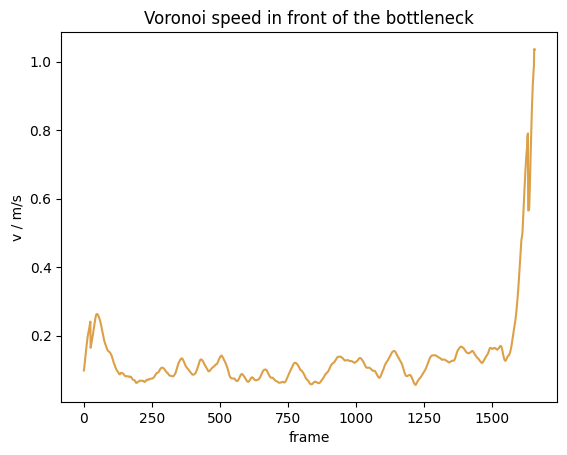
Voronoi speed#

A further approach to compute average speed \(v_{voronoi}(t)\) in an area by weighting the individuals speed by the size of their corresponding Voronoi polygon \(V_i\) inside the measurement area \(M\). The individuals speed are weighted by the proportion of their Voronoi cell \(V_i\) and the intersection with the measurement area \(V_i \cap M\).

The Voronoi speed \(v_{voronoi}(t)\) is defined as

\[ v_{voronoi}(t) = { \int\int v_{xy}(t) dxdy \over A(M)}, \]

where \(v_{xy}(t) = v_i(t)\) is the individual speed of each pedestrian, whose \(V_i(t) \cap M\) and \(A(M)\) the area of the measurement area.

Important

The Voronoi speed can only be computed when for each pedestrian inside the measurement area also a speed \(v_i(t)\) is computed, when using the exclude or adaptive approach this might not be the case. Then some extra processing steps are needed, to avoid this use the single sided approach.

This can be done in PedPy with:

from pedpy import compute_voronoi_speed

voronoi_speed = compute_voronoi_speed(
    traj_data=traj,
    individual_voronoi_intersection=intersecting,
    individual_speed=individual_speed_single_sided,
    measurement_area=measurement_area,
)

_images/b4789d6e4dfe5b56a8a22c2780ae45994a32189c9f762eb7d6b922d6564fea61.png

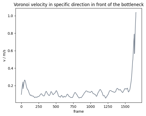
Analogously, this can be done with the speed in a specific direction with:

voronoi_speed_direction = compute_voronoi_speed(
    traj_data=traj,
    individual_voronoi_intersection=intersecting,
    individual_speed=individual_speed_direction,
    measurement_area=measurement_area,
)

_images/651d7c1f0cecb6aeed306254d1eb4f9782a3c8337e0b052c688b13413b631346.png

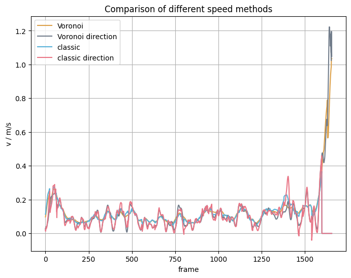
Comparison mean speed vs Voronoi speed#

We now computed the speed with different methods, this plot shows what the different results look like compared to each other:

_images/764d5d67cadf47b97a12465103b949915edc3c8e566389c0bb6ac681d848528c.png

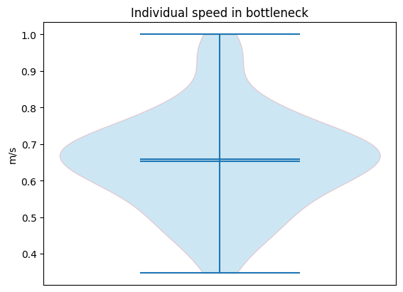
Passing speed (individual)#

With the same principles as described in passing density, the individual speeds \(v^i_{passing}\) is defined as

\[ v^i_{passing} = \frac{d}{t_{out}-t_{in}}, \]

where \(d\) is the distance between the two measurement lines.

In PedPy this can be done with:

from pedpy import compute_passing_speed
from pedpy import compute_frame_range_in_area

passing_offset = 1.0
frames_in_area, _ = compute_frame_range_in_area(
    traj_data=traj, measurement_line=measurement_line, width=passing_offset
)
passing_speed = compute_passing_speed(
    frames_in_area=frames_in_area,
    frame_rate=traj.frame_rate,
    distance=passing_offset,
)

_images/6ae1b262f4952654b02c0656442d395c638bf3443b728fec2b45c11caaf8f72c.png

Flow#

Another important metric, when analyzing pedestrian flows is the flow itself. It describes how many persons cross a line in a given time. From this potential bottlenecks or congestion can be derived.

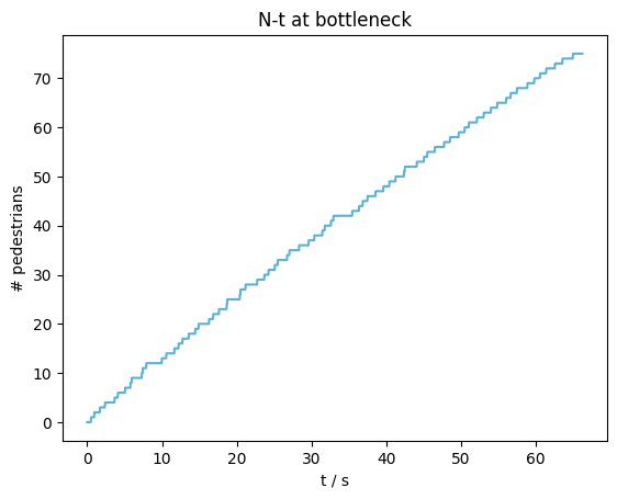
N-t diagram at bottleneck#

To get a first impression of the flow at the bottleneck we look at the N-t diagram, which shows how many pedestrian have crossed the measurement line at a specific time.

from pedpy import compute_n_t

nt, crossing = compute_n_t(
    traj_data=traj,
    measurement_line=measurement_line,
)

_images/c2257c374b93e5b17b3a0f7bbb9d4084ce3ff89eb7d3d175e95340748f56d274.png

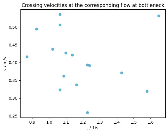
Flow at bottleneck#

From the N-t data we then can compute the flow at the bottleneck.

For the computation of the flow we look at frame intervals \(\Delta frame\) in which the flow is computed. The first intervals starts, when the first person crossed the measurement line. The next interval always starts at the time when the last person in the previous frame interval crossed the line.

In each of the time interval it is checked, if any person has crossed the line, if yes, a flow \(J\) can be computed. From the first frame the line was crossed \(f^{\Delta frame}_1\), the last frame someone crossed the line \(f^{\Delta frame}_N\) the length of the frame interval \(\Delta f\) can be computed:

\[ \Delta f = f^{\Delta frame}_N - f^{\Delta frame}_1 \]

This directly together with the frame rate of the trajectory \(fps\) gives the time interval \(\Delta t\):

\[ \Delta t = \Delta f / fps \]

Given the number of pedestrian crossing the line is given by \(N^{\Delta frame}\), the flow \(J\) becomes:

\[ J = \frac{N^{\Delta frame}}{\Delta t} \]

At the same time also the mean speed of the pedestrian when crossing the line is given by:

\[ v_{crossing} = {1 \over N^{\Delta t} } \sum^{N^{\Delta t}}_{i=1} v_i(t) \]

To compute the flow and mean speed when passing the line with PedPy use:

from pedpy import compute_flow

delta_frame = 100
flow = compute_flow(
    nt=nt,
    crossing_frames=crossing,
    individual_speed=individual_speed_single_sided,
    delta_frame=delta_frame,
    frame_rate=traj.frame_rate,
)

_images/91b2b8486abe77260f9d62fd988807423db60147ed9a8b8fd569196ec2ea1c38.png

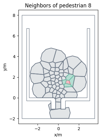
Neighborhood#

To analyze, which pedestrians are close to each other, it is possible to compute the neighbors of each pedestrian. We define two pedestrians as neighbors if their Voronoi polygons (\(V_i\), \(V_j\)) touch at some point, in case of PedPy they are touching if their distance is below 1mm. As basis for the computation one can either use the uncut or cut Voronoi polygons. When using the uncut Voronoi polygons, pedestrian may be detected as neighbors even when their distance is quite large in low density situation. Therefor, it is recommended to use the cut Voronoi polygons, where the cut-off radius can be used to define a maximal distance between neighboring pedestrians.

To compute the neighbors in PedPy use:

from pedpy import compute_neighbors

neighbors = compute_neighbors(individual_cutoff)

_images/7ff23db19d1d1cbd7488606a41618083c5d28fb6dc68a2c03240ee610f2b1f95.png

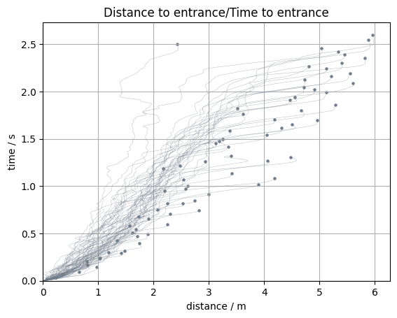
Distance to entrance/Time to entrance#

An indicator to detect congestions or jams in trajectory data are distance/time to crossing. It shows how much time until the crossing of the measurement line is left and how big the distance to that line is.

In PedPy this can be done with:

from pedpy import compute_time_distance_line

df_time_distance = compute_time_distance_line(
    traj_data=traj, measurement_line=measurement_line
)

_images/9cd4a4ff2eb6776d3d7a4bd2345504330d4a301eb18c211f8a96ed26a3a0671b.png

Profiles#

For the computation of the profiles the given walkable area is divided into square grid cells. Each of these grid cells is then used as a measurement area to compute the density and speed.

Note

As this is a quite compute heavy operation, it is suggested to reduce the trajectories to the important areas and limit the input data to the most relevant frame interval.

from pedpy import (
    compute_individual_voronoi_polygons,
    compute_individual_speed,
    SpeedCalculation,
    Cutoff,
)

individual_cutoff = compute_individual_voronoi_polygons(
    traj_data=traj,
    walkable_area=walkable_area,
    cut_off=Cutoff(radius=0.8, quad_segments=3),
)

individual_speed = compute_individual_speed(
    traj_data=traj,
    frame_step=5,
    speed_calculation=SpeedCalculation.BORDER_SINGLE_SIDED,
)

profile_data = individual_speed.merge(individual_cutoff, on=[ID_COL, FRAME_COL])
profile_data = profile_data.merge(traj.data, on=[ID_COL, FRAME_COL])

from pedpy import (
    get_grid_cells,
    compute_grid_cell_polygon_intersection_area,
)

grid_size = 0.4
grid_cells, _, _ = get_grid_cells(
    walkable_area=walkable_area, grid_size=grid_size
)

min_frame_profiles = 250  # We use here just an excerpt of the
max_frame_profiles = 400  # trajectory data to reduce compute time

profile_data = profile_data[
    profile_data.frame.between(min_frame_profiles, max_frame_profiles)
]

# Compute the grid intersection area for the resorted profile data (they have the same sorting)
# for usage in multiple calls to not run the compute heavy operation multiple times
(
    grid_cell_intersection_area,
    resorted_profile_data,
) = compute_grid_cell_polygon_intersection_area(
    data=profile_data, grid_cells=grid_cells
)

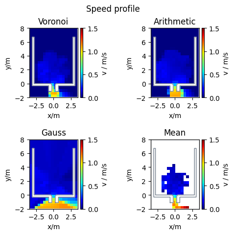
Speed Profiles#

This documentation describes the methods available for computing speed profiles within a specified area, focusing on pedestrian movements. Four distinct methods are detailed: Voronoi, Arithmetic, Mean, and Gauss speed profiles.

Voronoi speed profile

The Voronoi speed profile \(v_{\text{voronoi}}\) is computed from a weighted mean of pedestrian speeds. It utilizes the area overlap between a pedestrian’s Voronoi cell (\(V_i\)) and the grid cell (\(c\)). The weight corresponds to the fraction of the Voronoi cell residing within the grid cell, thereby integrating speed across this intersection:

\[ v_{\text{voronoi}} = { \int\int v_{xy} dxdy \over A(c)}, \]

where \(A(c)\) represents the area of the grid cell \(c\).

Arithmetic Voronoi speed profile

The arithmetic Voronoi speed \(v_{\text{arithmetic}}\) is computed as the mean of each pedestrian’s speed (\(v_i\)), whose Voronoi cell \(V_i\) intersects with grid cell \(c\):

\[ v_{\text{arithmetic}} = \frac{1}{N} \sum_{i \in V_i \cap P_c} v_i, \]

with \(N\) being the total number of pedestrians whose Voronoi cells overlap with grid cell \(c\).

Mean speed profile

The mean speed profile is computed by the average speed of all pedestrians \(P_c\) present within a grid cell \(c\):

\[ v_{\text{mean}} = \frac{1}{N} \sum_{i \in P_c} v_i \]

where \(N\) denotes the number of pedestrians in grid cell \(c\).

Gauss speed profiles

Calculates a speed profile based on Gaussian weights for an array of pedestrian locations and velocities. The speed, weighted at a grid cell \(c\) considering its distance \(\delta = \boldsymbol{r}_i - \boldsymbol{c}\) from an agent, is determined as follows:

\[ v_{\text{gauss}} = \frac{\sum_{i=1}^{N}{\big(w_i\cdot v_i\big)}}{\sum_{i=1}^{N} w_i}, \]

with \(w_i = \frac{1} {\sigma \cdot \sqrt{2\pi}} \exp\big(-\frac{\delta^2}{2\sigma^2}\big)\; \text{and}\; \sigma = \frac{FWHM}{2\sqrt{2\ln(2)}}. \)

from pedpy import compute_speed_profile, SpeedMethod

voronoi_speed_profile = compute_speed_profile(
    data=resorted_profile_data,
    walkable_area=walkable_area,
    grid_intersections_area=grid_cell_intersection_area,
    grid_size=grid_size,
    speed_method=SpeedMethod.VORONOI,
)

arithmetic_speed_profile = compute_speed_profile(
    data=resorted_profile_data,
    walkable_area=walkable_area,
    grid_intersections_area=grid_cell_intersection_area,
    grid_size=grid_size,
    speed_method=SpeedMethod.ARITHMETIC,
)

mean_speed_profile = compute_speed_profile(
    data=profile_data,
    walkable_area=walkable_area,
    grid_size=grid_size,
    speed_method=SpeedMethod.MEAN,
)

gauss_speed_profile = compute_speed_profile(
    data=profile_data,
    walkable_area=walkable_area,
    grid_size=grid_size,
    gaussian_width=0.5,
    speed_method=SpeedMethod.GAUSSIAN,
)

_images/b1985cb27ea2c73e8beb6c86772dfd0b20032b2b9c7930a69370b675bd90f7d0.png

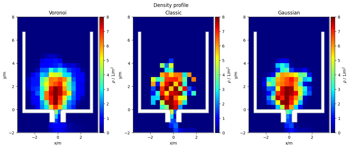
Density Profiles#

Currently, it is possible to compute either the Voronoi, classic or Gaussian density profiles.

Voronoi density profile

In each cell the Voronoi speed \(v_{voronoi}\) is defined as

\[ v_{voronoi}(t) = { \int\int v_{xy} dxdy \over A(M)}, \]

where \(v_{xy} = v_i\) is the individual speed of each pedestrian, whose \(V_i \cap M\) and \(A(M)\) the area the grid cell.

Classic density profile

In each cell the density \(\rho_{classic}\) is defined by

\[ \rho_{classic} = {N \over A(M)}, \]

where \(N\) is the number of pedestrians inside the grid cell \(M\) and the area of that grid cell (\(A(M)\)).

Gaussian density profile

In each cell the density \(\rho_{gaussian}\) is defined by

\[ \rho_{gaussian} = \sum_{i=1}^{N}{\delta (\boldsymbol{r}_i - \boldsymbol{c})}, \]

where \(\boldsymbol{r}_i\) is the position of a pedestrian and \(\boldsymbol{c}\) is the center of the grid cell. Finally \(\delta(x)\) is approximated by a Gaussian

\[ \delta(x) = \frac{1}{\sqrt{\pi}a}\exp[-x^2/a^2] \]

from pedpy import compute_density_profile, DensityMethod

# here it is important to use the resorted data, as it needs to be in the same ordering as "grid_cell_intersection_area"
voronoi_density_profile = compute_density_profile(
    data=resorted_profile_data,
    walkable_area=walkable_area,
    grid_intersections_area=grid_cell_intersection_area,
    grid_size=grid_size,
    density_method=DensityMethod.VORONOI,
)

# here the unsorted data can be used
classic_density_profile = compute_density_profile(
    data=profile_data,
    walkable_area=walkable_area,
    grid_size=grid_size,
    density_method=DensityMethod.CLASSIC,
)

gaussian_density_profile = compute_density_profile(
    data=profile_data,
    walkable_area=walkable_area,
    grid_size=grid_size,
    density_method=DensityMethod.GAUSSIAN,
    gaussian_width=0.5,
)

_images/2a2cc8ec8994dec11d7a76396549eadf03f93f61ef0c020d85b67012dc1ab12c.png

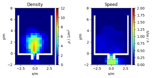
Density and Speed Profiles#

An other option is to compute both kinds of profile at the same time:

from pedpy import compute_profiles

min_frame_profiles = 250  # We use here just an excerpt of the
max_frame_profiles = 400  # trajectory data to reduce compute time
grid_size = 0.4

density_profiles, speed_profiles = compute_profiles(
    data=pd.merge(
        individual_cutoff[
            individual_cutoff.frame.between(
                min_frame_profiles, max_frame_profiles
            )
        ],
        individual_speed[
            individual_speed.frame.between(
                min_frame_profiles, max_frame_profiles
            )
        ],
        on=[ID_COL, FRAME_COL],
    ),
    walkable_area=walkable_area.polygon,
    grid_size=grid_size,
    speed_method=SpeedMethod.ARITHMETIC,
    density_method=DensityMethod.VORONOI,
)

_images/e732684f95d68a5f276fc8bb5859c73d61c086c436fd44c9ba3044adec77192c.png

Preprocess the data#

Until now, we used complete trajectories, but sometimes not all the data is relevant for the analysis. If the data comes from larger simulation or experiments you may be only interested in data close to your region of interest or data in a specific time range. As PedPy builds up on Pandas as data container, the filtering methods from Pandas can also be used here. More information on filtering and merging with Pandas can be found here: filtering & merging.

Geometric filtering#

First, we want to filter the data by geometrical principles, therefor we combine the capabilities of Pandas and Shapely.

Data inside Polygon#

In the first case, we are only interested in trajectory data inside the known measurement area.

import shapely

bottleneck = shapely.Polygon([(0.25, 0), (0.25, -1), (-0.25, -1), (-0.25, 0)])
leaving_area = shapely.Polygon([(-3, -1), (-3, -2), (3, -2), (3, -1)])

data_inside_ma = traj.data[shapely.within(traj.data.point, bottleneck)]

_images/b0f4b06eeb4a518fb92cc368b6c27ffbb8766efe79a325307e304140b2dd10ed.png

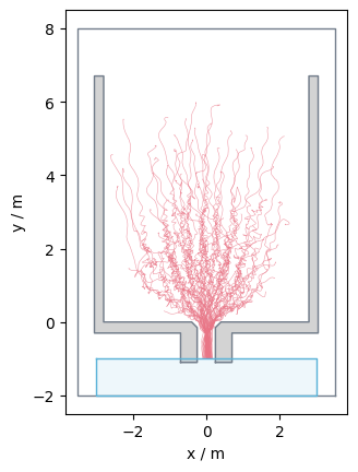
Data outside Polygon#

Secondly, we want to filter the data, such that the result contains only data which is outside a given area. In our case we want to remove all data behind the bottleneck, here called leaving area:

data_outside_leaving_area = traj.data[
    ~shapely.within(traj.data.point, leaving_area)
]

_images/225d620ed673f8ca2e6b714a7d72d8bdd0442ac5b5a113947852901b58389602.png

Data close to line#

It is not only possible to check whether a point is within a given polygon, it is also possible to check if the distance to a given geometrical object is below a given threshold. Here we want all the data that is within 1m of the measurement line at the entrance of the bottleneck:

data_close_ma = traj.data[
    shapely.dwithin(traj.data.point, measurement_line.line, 1)
]

_images/1c76c6a57857f4e69e92181a75dd8c375143efe6b04388838b288793596cf888.png

Time based filtering#

It is not only possible to filter the data by geometrical means, but also depending on time information. In experiments, you might only be interested in steady state data, this can be also be achieved by slicing the data:

traj_data_frame_range = traj[300:600]

_images/fd1775f06609e3fb20b63d195e734f99d27d3276bae9ac621413d5603fc4ad9a.png

Alternatively, you could also utilise the Pandas filtering methods:

data_frame_range = traj.data[
    traj.data.frame.between(300, 600, inclusive="both")
]

_images/4778b192ee4152e998f39bbd76db96f19012a29a9b97712915dae8aa518ed9db.png

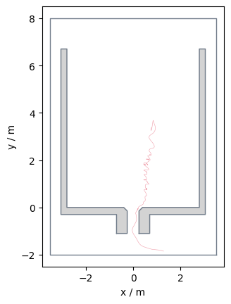
ID based filtering#

It is also possible to filter the data in a way that only specific pedestrians are contained:

data_id = traj.data[traj.data.id == 20]

_images/99f92a1d0d709bda8b1b0eb2a9fe707ba3a845c33827b7b8a35d34a2c9e1afc2.png

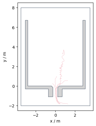
It is also possible to filter for multiple ids:

ids = [10, 20, 30, 40]
data_id = traj.data[traj.data.id.isin(ids)]

_images/2913e4eeec1a42f573acd4d73a52a629b48fa3ae47a734c0fefa8000bb4968cc.png

What to do with the results?#

Now we have completed our analysis, what can be done to

access specific columns
combine for further analysis
save results

Access specific columns#

In order to access a specific column of the computed results or the trajectory data PedPy provides all the column names for access. It is highly encouraged to use these identifiers instead of using the column names directly, as the identifier would be updated, if they change. A list of all identifiers can be found in the API reference.

from pedpy.column_identifier import *

# Access with column identifier
traj.data[[ID_COL, FRAME_COL, POINT_COL]]

	id	frame	point
0	1	0	POINT (2.1569 2.659)
1	1	1	POINT (2.1498 2.6653)
2	1	2	POINT (2.1532 2.6705)
3	1	3	POINT (2.1557 2.6496)
4	1	4	POINT (2.1583 2.6551)
...	...	...	...
63105	75	492	POINT (0.1539 -1.5997)
63106	75	493	POINT (0.1792 -1.6365)
63107	75	494	POINT (0.2262 -1.704)
63108	75	495	POINT (0.2575 -1.7516)
63109	75	496	POINT (0.2885 -1.8041)

63110 rows × 3 columns

# Access with column names
traj.data[["id", "frame", "point"]]

	id	frame	point
0	1	0	POINT (2.1569 2.659)
1	1	1	POINT (2.1498 2.6653)
2	1	2	POINT (2.1532 2.6705)
3	1	3	POINT (2.1557 2.6496)
4	1	4	POINT (2.1583 2.6551)
...	...	...	...
63105	75	492	POINT (0.1539 -1.5997)
63106	75	493	POINT (0.1792 -1.6365)
63107	75	494	POINT (0.2262 -1.704)
63108	75	495	POINT (0.2575 -1.7516)
63109	75	496	POINT (0.2885 -1.8041)

63110 rows × 3 columns

Combine multiple DataFrames#

From the analysis we have one DataFrame containing the trajectory data:

traj.data

	id	frame	x	y	point
0	1	0	2.1569	2.6590	POINT (2.1569 2.659)
1	1	1	2.1498	2.6653	POINT (2.1498 2.6653)
2	1	2	2.1532	2.6705	POINT (2.1532 2.6705)
3	1	3	2.1557	2.6496	POINT (2.1557 2.6496)
4	1	4	2.1583	2.6551	POINT (2.1583 2.6551)
...	...	...	...	...	...
63105	75	492	0.1539	-1.5997	POINT (0.1539 -1.5997)
63106	75	493	0.1792	-1.6365	POINT (0.1792 -1.6365)
63107	75	494	0.2262	-1.7040	POINT (0.2262 -1.704)
63108	75	495	0.2575	-1.7516	POINT (0.2575 -1.7516)
63109	75	496	0.2885	-1.8041	POINT (0.2885 -1.8041)

63110 rows × 5 columns

and one containing the individual Voronoi data:

individual

	id	frame	polygon	density
0	1	0	POLYGON ((1.7245255133043016 2.849134813766198...	1.323393
979	2	0	POLYGON ((1.5217781622975501 1.153757147573504...	1.212123
1347	3	0	POLYGON ((1.7425304074633392 1.895950902917607...	2.046083
2011	4	0	POLYGON ((1.7425304074633392 1.895950902917607...	1.969356
2707	5	0	POLYGON ((1.2090226182277728 1.025737783544312...	1.094197
...	...	...	...	...
57481	69	1652	POLYGON ((-3.5 -2, -3.5 8, 3.5 8, 3.5 -2, -3.5...	0.015559
57482	69	1653	POLYGON ((-3.5 -2, -3.5 8, 3.5 8, 3.5 -2, -3.5...	0.015559
57483	69	1654	POLYGON ((-3.5 -2, -3.5 8, 3.5 8, 3.5 -2, -3.5...	0.015559
57484	69	1655	POLYGON ((-3.5 -2, -3.5 8, 3.5 8, 3.5 -2, -3.5...	0.015559
57485	69	1656	POLYGON ((-3.5 -2, -3.5 8, 3.5 8, 3.5 -2, -3.5...	0.015559

63110 rows × 4 columns

As both have the columns ‘id’ and ‘frame’ in common, these can be used to merge the dataframes. See pandas.merge() and pandas.DataFrame.merge() for more information on how DataFrames can be merged.

data_with_voronoi_cells = traj.data.merge(intersecting, on=[ID_COL, FRAME_COL])
data_with_voronoi_cells

	id	frame	x	y	point	polygon	density	intersection
0	1	0	2.1569	2.6590	POINT (2.1569 2.659)	POLYGON ((1.7245255133043016 2.849134813766198...	1.323393	POLYGON EMPTY
1	1	1	2.1498	2.6653	POINT (2.1498 2.6653)	POLYGON ((1.7360824366848313 2.862174491143732...	1.334515	POLYGON EMPTY
2	1	2	2.1532	2.6705	POINT (2.1532 2.6705)	POLYGON ((1.8536919501780398 2.459236372880033...	1.328666	POLYGON EMPTY
3	1	3	2.1557	2.6496	POINT (2.1557 2.6496)	POLYGON ((1.7354793571480895 2.853885114270424...	1.344024	POLYGON EMPTY
4	1	4	2.1583	2.6551	POINT (2.1583 2.6551)	POLYGON ((1.7364457387060401 2.854024613400598...	1.349853	POLYGON EMPTY
...	...	...	...	...	...	...	...	...
63105	75	492	0.1539	-1.5997	POINT (0.1539 -1.5997)	POLYGON ((3.5 -1.55952287010524, 3.5 -2, -3.18...	0.198106	POLYGON EMPTY
63106	75	493	0.1792	-1.6365	POINT (0.1792 -1.6365)	POLYGON ((1.4972019470076683 -0.88399685153128...	0.204326	POLYGON EMPTY
63107	75	494	0.2262	-1.7040	POINT (0.2262 -1.704)	POLYGON ((1.5304646340900363 -0.88904050056830...	0.216082	POLYGON EMPTY
63108	75	495	0.2575	-1.7516	POINT (0.2575 -1.7516)	POLYGON ((1.5619810613615523 -0.89649921050952...	0.227548	POLYGON EMPTY
63109	75	496	0.2885	-1.8041	POINT (0.2885 -1.8041)	POLYGON ((1.5948468195234426 -0.90689232729486...	0.241937	POLYGON EMPTY

63110 rows × 8 columns

from pedpy.column_identifier import SPEED_COL

data_with_voronoi_cells_speed = data_with_voronoi_cells.merge(
    individual_speed[[ID_COL, FRAME_COL, SPEED_COL]], on=[ID_COL, FRAME_COL]
)
data_with_voronoi_cells_speed

	id	frame	x	y	point	polygon	density	intersection	speed
0	1	0	2.1569	2.6590	POINT (2.1569 2.659)	POLYGON ((1.7245255133043016 2.849134813766198...	1.323393	POLYGON EMPTY	0.055227
1	1	1	2.1498	2.6653	POINT (2.1498 2.6653)	POLYGON ((1.7360824366848313 2.862174491143732...	1.334515	POLYGON EMPTY	0.142829
2	1	2	2.1532	2.6705	POINT (2.1532 2.6705)	POLYGON ((1.8536919501780398 2.459236372880033...	1.328666	POLYGON EMPTY	0.191291
3	1	3	2.1557	2.6496	POINT (2.1557 2.6496)	POLYGON ((1.7354793571480895 2.853885114270424...	1.344024	POLYGON EMPTY	0.215515
4	1	4	2.1583	2.6551	POINT (2.1583 2.6551)	POLYGON ((1.7364457387060401 2.854024613400598...	1.349853	POLYGON EMPTY	0.277554
...	...	...	...	...	...	...	...	...	...
63105	75	492	0.1539	-1.5997	POINT (0.1539 -1.5997)	POLYGON ((3.5 -1.55952287010524, 3.5 -2, -3.18...	0.198106	POLYGON EMPTY	0.895094
63106	75	493	0.1792	-1.6365	POINT (0.1792 -1.6365)	POLYGON ((1.4972019470076683 -0.88399685153128...	0.204326	POLYGON EMPTY	0.947931
63107	75	494	0.2262	-1.7040	POINT (0.2262 -1.704)	POLYGON ((1.5304646340900363 -0.88904050056830...	0.216082	POLYGON EMPTY	1.192062
63108	75	495	0.2575	-1.7516	POINT (0.2575 -1.7516)	POLYGON ((1.5619810613615523 -0.89649921050952...	0.227548	POLYGON EMPTY	1.306230
63109	75	496	0.2885	-1.8041	POINT (0.2885 -1.8041)	POLYGON ((1.5948468195234426 -0.90689232729486...	0.241937	POLYGON EMPTY	1.426141

63110 rows × 9 columns

Save in files#

For preserving the results on the disk, the results need to be saved on the disk. This can be done with the build-in functions from Pandas.

Create directories to store the results#

First we create a directory, where we want to save the results. This step is optional!

pathlib.Path("results_introduction/profiles/speed").mkdir(
    parents=True, exist_ok=True
)
pathlib.Path("results_introduction/profiles/density").mkdir(
    parents=True, exist_ok=True
)

results_directory = pathlib.Path("results_introduction")

Save Pandas DataFrame (result from everything but profiles) as csv#

Now, a DataFrame can be saved as csv with:

from pedpy.column_identifier import (
    X_COL,
    Y_COL,
    DENSITY_COL,
    INTERSECTION_COL,
    POLYGON_COL,
)
import csv

with open(
    results_directory / "individual_result.csv", "w"
) as individual_output_file:
    individual_output_file.write(f"#framerate:	{traj.frame_rate}\n\n")
    data_with_voronoi_cells_speed[
        [
            ID_COL,
            FRAME_COL,
            X_COL,
            Y_COL,
            DENSITY_COL,
            SPEED_COL,
            POLYGON_COL,
            INTERSECTION_COL,
        ]
    ].to_csv(
        individual_output_file,
        mode="a",
        header=True,
        sep="\t",
        index_label=False,
        index=False,
        quoting=csv.QUOTE_NONNUMERIC,
    )

Save numpy arrays (result from profiles) as txt#

The profiles are returned as Numpy arrays, which also provide a build-in save function, which allows to save the arrays as txt format:

results_directory_density = results_directory / "profiles/density"
results_directory_speed = results_directory / "profiles/speed"

for i in range(len(range(min_frame_profiles, min_frame_profiles + 10))):
    frame = min_frame_profiles + i
    np.savetxt(
        results_directory_density / f"density_frame_{frame:05d}.txt",
        density_profiles[i],
    )
    np.savetxt(
        results_directory_speed / f"speed_frame_{frame:05d}.txt",
        speed_profiles[i],
    )

User Guide

Contents

User Guide#

Analysis set-up#

Walkable area#

Prepare measurement details#

Importing pedestrian movement data#

Loading from Pandas DataFrame#

Loading from text trajectory files#

Loading from hdf5 trajectory files#

Loading from Viswalk trajectory files#

Plot setup#

Validate that trajectory is completely inside the walkable area.#

Analysis#

Density#

Classic density#

Voronoi density#

Compute individual Voronoi Polygons#

Without cut-off#

With cut-off#

Comparison#

Compute actual Voronoi density#

Without cut-off#

With cut-off#

Comparison#

Passing density (individual)#

Speed#

Individual speed#

Exclude border#

Adaptive border window#

Single sided border window#

Comparison#

Individual speed in specific movement direction#

Mean speed#

Voronoi speed#

Comparison mean speed vs Voronoi speed#

Passing speed (individual)#

Flow#

N-t diagram at bottleneck#

Flow at bottleneck#

Neighborhood#

Distance to entrance/Time to entrance#

Profiles#

Speed Profiles#

Density Profiles#

Density and Speed Profiles#

Preprocess the data#

Geometric filtering#

Data inside Polygon#

Data outside Polygon#

Data close to line#

Time based filtering#

ID based filtering#

What to do with the results?#

Access specific columns#

Combine multiple DataFrames#

Save in files#

Create directories to store the results#

Save Pandas DataFrame (result from everything but profiles) as csv#

Save numpy arrays (result from profiles) as txt#